In this post I want to describe how I created a CFD diagram in Excel based on tickets with timestamps. A team that I coach puts a date on their tickets when they enter various steps on their Kanban board and we then add this data to a CFD . I assume that you are familiar with cumulative flow charts. If not, I’d suggest reading the following book Actionable Agile Metrics for Predictability: An Introduction.

The problem

Why don’t I take something that is already there? My team uses a paper board and I could not find (free) examples that work with timestamps instead of counting the items in columns. Let me explain that with the following picture:

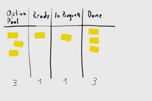
If I count the items on the board (3 items in option pool, 1 in ready,…) in every column every day during the standup for example I can collect this data in an Excel sheet and create a CFD diagram out of it easily. You can find an explanation for this method for example in this blog post.

A better approach is to put dates on the tickets when they enter a state you want to track. This approach is better because you can put further analysis on this data which you can’t when you only count the items. Also, you … no, wait: please read the book by Vacanti. That’s not my job here.

I found the following web tools for analysis https://actionableagile.com. You can import an Excel sheet or connect Jira and you get the CFD and further analysis out of the box, but it costs something. I thought that a masters degree in computer science should qualify me for creating an Excel sheet for myself.

So here it is:

The solution

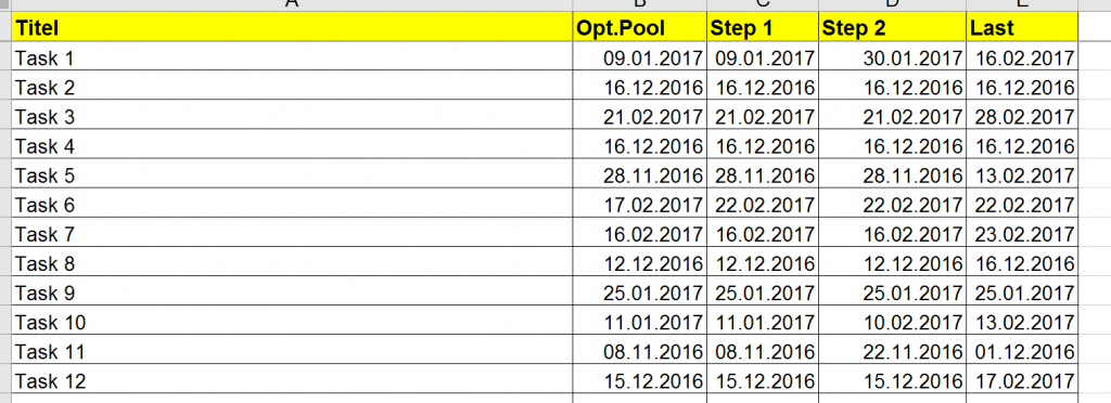
The first sheet in my Excel sheet contains the board input data.

 

 

 

 

The second sheet now creates the table as basis for the CFD diagram:

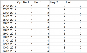
You need to span the timerange you want in the first column. Here you can also decide if you want to have the CFD on a daily, weekly or monthly basis. The formula does the rest.

When you go right in every row you see how many items have been in a certain state on the date of that row. On July 1st, we had 1 in option pool, 2 in Step 1, 2 in Step 2 and 0 Last.

Here is the formula for counting items:

=COUNTIFS(InputData!B:B;"<="&TimeRange!A2;InputData!C:C;">"&A2)

Count all items where the time in the state we are looking at (for example option pool) is smaller or equal to the current date we are looking at (for example July 1st) and only take those items that have a date in the next state that is greater than the current date.

So, for example we see a ticket with a ready timestamp of July 1st and it has a “Step 1” timestamp on July 3rd. This counts as item in the ready column from July 1st until July 3rd, because from July 3rd on this item is then in “Step 1”.

I have a different formula for the “Last” state or in general the departure state of our diagram, because I just wanted to count the items that have been finished after the begin date of our timerange and there is no state after “Last” of course.

=COUNTIFS(InputData!E:E;"<="&TimeRange!A2;InputData!E:E;">"&$A$2)

Now just copy this formulas into every row (just make sure that you always refer to the first column when you copy the formulas to right cells).

The last step is to create the chart.

Just mark the whole table and insert a “Stacked Area” diagram. Make sure that the arrival column (in our example “Opt. Pool”) is shown on top and the departure column (“Last”) is on the bottom. It is basically the same now as from step 14 in this blog post.

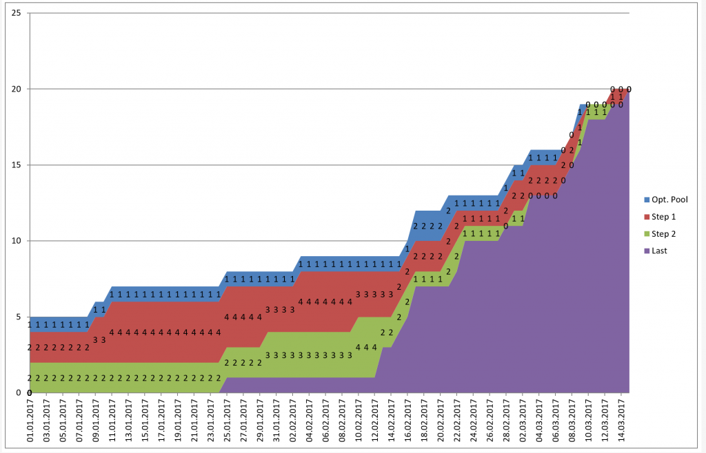
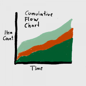
The resulting CFD then looks like this. You can always cross-check your CFD by using the actionableagile.com tools.

The resulting Excel

You can download an example sheet here: Kanban_CFD

References

Vacanti, 2015. Actionable Agile Metrics for Predictability, ActionableAgile Press